Finite Element Implementation

The implementation of the CVFE scheme relies on the following form of the principle of virtual work:

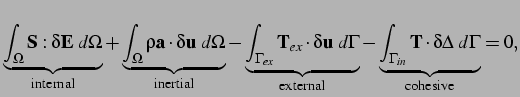$$\underbrace{\int_{\Omega} {\bf S} : \delta {\bf E} \,\, d\Omega}_... ... \delta\boldsymbol{\Delta} \,\,d\Gamma}_{\textrm{cohesive}} = 0,\vspace*{0.5cm}$$ (2.6)

where $\Omega$ is the undeformed domain, $\Gamma_{in}$ denotes the interior ``cohesive'' boundary along which the cohesive tractions ${\bf T}$ act, and $\Gamma_{ex}$ corresponds to the part of the exterior boundary along which the external tractions ${\bf T}_{ex}$ are applied. ${\bf a}$ and ${\bf u}$ denote the acceleration and displacement fields, respectively. ${\bf S}$ is the second Piola-Kirchoff stress tensor and ${\bf E}$, the Lagrangian strain tensor, which is related to the displacement field through

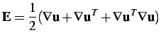$${\bf E} = \frac{1}{2} ( \nabla {\bf u} + \nabla {\bf u}^T + \nabla {\bf u}^T \nabla {\bf u} )$$ (2.7)

Nonlinear kinematics is used in this study to account for the possible large rotations present in the structure due to the fracture process. The expression (2.6) of the principle of virtual work is fairly conventional, except for the presence of the fourth term, which corresponds to the virtual work done by cohesive traction ${\bf T}$ for a virtual separation $\delta{\bf\Delta}$.

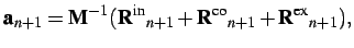
The resulting semi-discrete finite element formulation can be expressed in the following matrix form:

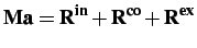$${\bf M}{\bf a} = {\bf R}^{\bf in} +{\bf R}^{\bf co} +{\bf R}^{\bf ex}$$ (2.8)

where ${\bf M}$ is the lumped mass matrix, ${\bf a}$ is the vector containing the nodal accelerations, and ${\bf R}^{\bf in}$, ${\bf R}^{\bf co}$ and ${\bf R}^{\bf ex}$ respectively denote the internal, cohesive and external force vectors.

The time stepping scheme is based on the classical explicit second-order central difference scheme (Belytschko et al., 1976):

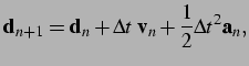$${\bf d}_{n+1} = {\bf d}_n + \Delta t \,\, {\bf v}_n + \frac{1}{2} \Delta t^2 {\bf a}_n,$$ (2.9)

$${\bf a}_{n+1} = {\bf M}^{-1}({{\bf R}^\textrm{in}}_{n+1} + {{\bf R}^\textrm{co}}_{n+1} + {{\bf R}^\textrm{ex}}_{n+1}),$$ (2.10)

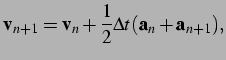$${\bf v}_{n+1} = {\bf v}_n +\frac{1}{2} {\Delta t} ({\bf a}_n + {\bf a}_{n+1}), \vspace*{0.5cm}$$ (2.11)

where $\Delta t$ is the time step and ${\bf d}_{n}$ denotes the nodal displacement vector at time $n \Delta t$.

The expression of the internal, cohesive and external force vectors can be found in Baylor (1997).While a variety of constitutive models can be used to characterize the response of the volumetric elements, we use, in this study, a simple linear isotropic relation between the second Piola-Kirchoff stresses ${\bf S}$ and the Lagrangian strains ${\bf E}$:

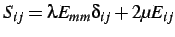$$S_{ij} = \lambda E_{mm} \delta_{ij} + 2 \mu E_{ij}$$ (2.12)

where $\lambda$ and $\mu$ are the Lame's constants.