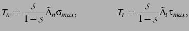
As mentioned above, the backbone of this research is the CVFE scheme, which is schematically presented in Figure 2.1. It consists of a combination of conventional (volumetric) elements (represented by 3-node triangles in Figure 2.1, although most types of structural finite elements can be used) and of interfacial (cohesive) elements (represented by a 4-node element in Figure 2.1, although higher-order cohesive elements are also available). The volumetric elements are used to characterize the mechanical response of the bulk material, while the cohesive elements are introduced in the finite element mesh to simulate the spontaneous motion of one or more cracks in the structure. The capture of the failure process is achieved with the aid of a phenomenological cohesive failure law characterizing the evolution of the cohesive element response.
![\includegraphics[scale=0.5]{cstelem.eps}](img54.png)
|
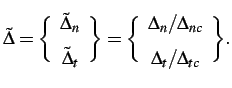
The choice of the cohesive failure model plays an important role in
the simulation of the fracture process. In this study, we use the
bilinear rate-independent intrinsic formulation introduced by
Geubelle and Baylor (1998), which is presented in
Figure 2.2 for the
pure mode I and mode II cases. The cohesive relation consists in two
distinct portions: a linearly rising part, indicating an increasing
resistance of the cohesive element to the separation of the adjacent
volumetric elements, followed by a monotonically decreasing relation
between cohesive traction and displacement jump simulating the
progressive failure of the material. The maximum value of the normal
(
![]() ) and tangential (
) and tangential (
![]() ) cohesive tractions respectively
correspond to tensile and shear strengths of the material. Once the
displacement jump (
) cohesive tractions respectively
correspond to tensile and shear strengths of the material. Once the
displacement jump (![]() for the tensile case and
for the tensile case and ![]() for the
shear case) has reached a critical value (respectively denoted by
for the
shear case) has reached a critical value (respectively denoted by
![]() and
and
![]() for the mode I and II
cases in Figure 2.2), the
cohesive traction is assumed to vanish. No more mechanical
interaction is then assumed to take place between the initially
adjacent volumetric elements, thereby creating a traction-free
surface (i.e., a crack) in the discretized solid domain.
for the mode I and II
cases in Figure 2.2), the
cohesive traction is assumed to vanish. No more mechanical
interaction is then assumed to take place between the initially
adjacent volumetric elements, thereby creating a traction-free
surface (i.e., a crack) in the discretized solid domain.
![\includegraphics[scale=0.40]{cohesive.eps}](img59.png)
|
The area under the cohesive traction/separation curve correspond to
the energy needed to generate a new fracture surface, i.e., the
fracture toughness of the material, denoted by ![]() and
and ![]() for the
modes I and II, respectively. To account for the possible coupling
between the failure modes, the normal and tangential cohesive
tractions,
for the
modes I and II, respectively. To account for the possible coupling
between the failure modes, the normal and tangential cohesive
tractions, ![]() and
and ![]() , are related to the norm of the displacement
jump vector
, are related to the norm of the displacement
jump vector
![]() through the introduction of the
residual strength parameter
through the introduction of the
residual strength parameter ![]() defined as
defined as
 |
(2.2) |
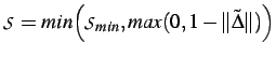
To limit the detrimental effect that the compliance of the cohesive
elements might have on the stress field solution, the residual
strength parameter of a cohesive element is initially given a value
![]() very close to unity. Typically a value of
very close to unity. Typically a value of ![]() to
to ![]() is used. As the element fails, this value progressively
decreases to zero, at which point complete failure is assumed to have
occurred. In order to maintain a monotonic decrease of this strength
parameter and thereby prevent the possible healing of the cohesive
elements, the minimum value achieved by
is used. As the element fails, this value progressively
decreases to zero, at which point complete failure is assumed to have
occurred. In order to maintain a monotonic decrease of this strength
parameter and thereby prevent the possible healing of the cohesive
elements, the minimum value achieved by
![]() is stored at each
integration point by using
is stored at each
integration point by using
 |
(2.3) |
The resulting rate-independent coupled bilinear cohesive traction-separation law can be expressed as
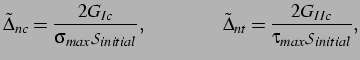 |
(2.5) |
![\includegraphics[scale=0.85]{normal3d.eps}](img77.png)
![\includegraphics[scale=0.85]{shear3d.eps}](img78.png)
|