Using a uniform time step in non-uniform meshes is a very costly and inefficient. The extensive research on the topic of time step optimization has led to the development of various multi-time step subcycling algorithms. The initial work of Belytschko and Mullen in 1976 led to an ``implicit-explicit'' method for second order equations using nodal partitioning (Neal and Belytschko, 1998). Further research, by Hughes and Lui (1978), led to a ``implicit-explicit'' subcycling method using element partitioning. In our research we have adopted an explicit subcycling method for second order equations presented by Smolinski (1989). This algorithm allows the use of different time steps in different regions of the same problem. As a result, we are not constrained by the minority elements, rather each region is given a time step that maximizes its efficiency while still satisfying the local Courant condition. This has the added benefit of minimizing the number of calculations necessary in the larger time step regions over the same time period. Multi-time step methods partition a mesh with different time steps using either nodal or element partitioning. The algorithm presented by Smolinski employs nodal partitioning. For nodal partitioning, time steps are distributed to nodes or nodal groups, while in element partitioning, the elements themselves are given different time steps.
Although the algorithm presented by Smolinski is capable of
supporting multiple time step regions, we have decided, for
simplicity reason, to limit the number of regions to only two -
designated as regions ![]() and
and ![]() . It should be noted that the nodes of
the two regions are not restricted to be grouped together, instead
they can be dispersed over the entire mesh as is shown in
Figure 2.5.
. It should be noted that the nodes of
the two regions are not restricted to be grouped together, instead
they can be dispersed over the entire mesh as is shown in
Figure 2.5.
For our analysis, we designate region ![]() as the critical region,
having the smaller time step equal to
as the critical region,
having the smaller time step equal to
![]() . This region
encompasses the smaller volumetric elements as well as any cohesive
elements in the system. Region
. This region
encompasses the smaller volumetric elements as well as any cohesive
elements in the system. Region ![]() is given a time step of
is given a time step of
![]() , where the subcycling parameter,
, where the subcycling parameter, ![]() , is thus the ratio of time
steps from region
, is thus the ratio of time
steps from region ![]() to region
to region ![]() . If
. If ![]() , all regions are given an
equal time step and no subcycling is performed. When subcycling is
used, this time step ratio must always be a positive even number.
, all regions are given an
equal time step and no subcycling is performed. When subcycling is
used, this time step ratio must always be a positive even number.
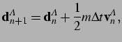
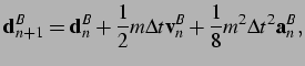
Once the nodal partitioning has been performed for the initial mesh,
the subcycling algorithm is directly applied to the central
difference time stepping loop. As the solution is stepped from time
![]() to time
to time
![]() , the nodes of region
, the nodes of region ![]() are updated
are updated ![]() times using the standard discretization equations. Region
times using the standard discretization equations. Region ![]() , on the
other hand, is the subcycled region over the same time period, to
which an approximate method is applied. Region
, on the
other hand, is the subcycled region over the same time period, to
which an approximate method is applied. Region ![]() is not explicitly
updated, rather the nodal accelerations of region
is not explicitly
updated, rather the nodal accelerations of region ![]() are toggled after
each time
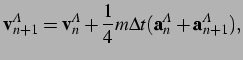
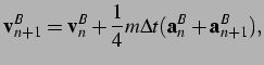
step. Since the parameter
are toggled after
each time
step. Since the parameter ![]() is even and since the nodal velocity
update is of the form
is even and since the nodal velocity
update is of the form
![]() , alternating the sign of the acceleration has for
effect to keep the velocity constant in region
, alternating the sign of the acceleration has for
effect to keep the velocity constant in region ![]() . This toggling of
nodal accelerations in
region
. This toggling of
nodal accelerations in
region ![]() foregoes the calculation of the internal and cohesive forces,
thereby saving a significant portion of time that would normally be
dedicated to these calculations. The equations used for direct calculations
in region
foregoes the calculation of the internal and cohesive forces,
thereby saving a significant portion of time that would normally be
dedicated to these calculations. The equations used for direct calculations
in region ![]() and approximations in region
and approximations in region ![]() are thus given by
are thus given by
Since the internal force calculations are performed by assembling the
local internal force vectors obtained for all the volumetric
elements, the most efficient way to take advantage of the subcycling
scheme is by flagging the volumetric elements based on the type of
nodes (![]() or
or ![]() ) they contain. This allows to quickly ``pass by'' all the
elements containing nodes of type
) they contain. This allows to quickly ``pass by'' all the
elements containing nodes of type ![]() during the first
during the first ![]() time steps
of the subcycling loop. In the implementation adopted in the present
work, all elements of type
time steps
of the subcycling loop. In the implementation adopted in the present
work, all elements of type ![]() have a flag of
have a flag of ![]() , all those of type
, all those of type ![]() have a flag of
have a flag of ![]() , and all those of ``mixed type'' (i.e., which
contain some nodes of type
, and all those of ``mixed type'' (i.e., which
contain some nodes of type ![]() and some of type
and some of type ![]() ) receive a flag of
) receive a flag of
![]() . This flag then insures that internal force calculations are
performed only on those elements having the a flag of
. This flag then insures that internal force calculations are
performed only on those elements having the a flag of ![]() or
or ![]() ,
corresponding to elements having at least one node from region
,
corresponding to elements having at least one node from region ![]() . The
computational savings we achieve are equal to the number of elements
having a flag of
. The
computational savings we achieve are equal to the number of elements
having a flag of ![]() , i.e. elements whose internal force calculation
is skipped. Figure 2.6 shows an example of
applying the element time step flags to a typical mesh.
, i.e. elements whose internal force calculation
is skipped. Figure 2.6 shows an example of
applying the element time step flags to a typical mesh.
An added benefit of the subcycling algorithm is that it can be
readily implemented in an adaptive fashion. The time steps of the
individual nodes, as well as of the volumetric elements, can be
changed at any time during the simulation. This allows the mesh to
adapt to the changing critical region. When used in conjunction with
adaptive meshing, the time steps are reduced as the local mesh is
made finer, and increased as the mesh grows coarser. With dynamic
cohesive element insertion, the time steps decrease as cohesive
elements are inserted.
|
![\includegraphics[scale=0.7]{subregions.eps}](img117.png)
![\includegraphics[scale=0.6]{timesteps.eps}](img140.png)