Computational Efficiency

A good representation of the efficiency of the parallel solution is to observe the parallel speedup of the code, given by

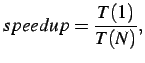$$speedup = \frac{T(1)}{T(N)},$$ (2.35)

where $T(1)$ is the time required to run the simulation on one processor, and $T(N)$ is the time required to run this same simulation on $N$ processors. With this we can track how well the code is able to perform when distributed across multiple processors. Ideally, we would prefer to have perfect speedup, where the solution time is decreased in proportion to the number of processors. Unfortunately, the speedup of most simulations begins to decrease with an increasing number of processors. This is because the cost of the parallelization becomes greater relative to the cost of the computations performed by each processor. Eventually, for many processors, the communication between them dominates the total time of the solution.