1D Transient Finite Element Method

for Thermal Problems and Structural Problems

AAE 320 – Project 3

Mariusz Zaczek

May 7, 2000

1.0 Introduction

The finite element method is a numerical procedure to evaluate various problems such as heat transfer, fluid flow, stress analysis, etc. An important aspect of the analysis is the ability to see the affect on a structure over time - referred to as "transient" problems. Two thermal and structural problems in one dimension have been analyzed below.

2.0 1D Transient Thermal Problem

2.1 Theory

The transient thermal problem is evaluated using the direct integration method. The primary finite element equation is the second order direct integration equation:

(1)

Transient thermal problems are first order so the acceleration term is not necessary. After some manipulations the resulting equation used for the problem is:

(2)

In order to solve the transient thermal problem an initial temperature field is required for time t=0. The temperature at t=Dt is obtained from the solution of the above equation. This new solution becomes the input to the solution for time t=2*Dt. It is assumed that the heat conduction matrix [C] and the internal heat generation vector {R} are constant over time. The use of BETA in the equation enables the user to select the type of scheme to use for the direct integration method. The BETA value itself will in part determine the stability of the solution. The table below lists some example BETA values and the schemes they represent.

Table 1. Beta Schemes

b = 0	forward difference or Euler (conditionally stable)
b >= 1/2	(unconditionally stable)
b = 1/2	Crank-Nicolson or trapezoidal rule (unconditionally stable)
b = 2/3	Galerkin (unconditionally stable)
b = 1	Backward difference (unconditionally stable)

Depending on which b is used, the time step used may also affect stability. For example if b ‘ 1/2 then the scheme used is unconditionally stable and thus any time step can be used and still maintain stability of the result. Using a smaller time step will make the solution more accurate even for unconditionally stable schemes. When the scheme is only conditionally stable then the affect of the time step is very large. To calculate the upper limit of the time step to be used one must first determine the largest eigenvalue and use the following equation:

(3)

In addition, if b is equal to zero the algorithm is explicit. Explicit methods are much easier to solve assuming the matrix [C] is diagonal. If b > 0, then the algorithm is implicit. Implicit methods require the knowledge of time derivatives of the temperature for one time step in the future, explicit method only require the derivatives of the temperature for the current time step.

2.2 Code Implementation

The transient thermal algorithm was implemented in one-dimension. The user is required to select a structure consisting of several elements. Each element is defined by several constant values such as density, length, thermal conductivity, specific heat, and a value for the internal heat generation. In addition the user can specify that any node have a constant heat source as a boundary condition. The other key inputs include the number of time steps over which to evaluate the problem, the time step to use and the b value. A step increment variable tells the program at which time step increment to output data into a file for future evaluation.

A copy of the actual code is attached to the back of this paper.

2.3 Graphical User Interface

The thermal program has a separate graphical user interface in which the user can specify the 1D field and any boundary condition.

Figure 1: Graphical User Interface for 1D Transient Thermal Code

The interface is called display_thermal.tcl and can either be started with the command: wish display_thermal.tcl or if the file is “executable” then simply typing display_thermal.tcl will bring up the program. The user can quit by simply selecting “quit” from the pull down “file” menu. The first step in a thermal analysis is the selection of the number of time steps to be used as well as the b and Dt values. Next, the actual structure is defined by entering elemental information into the appropriate boxes. The “From elem” box will specify the first element and the “To elem” box specifies the final element of a series. The length, density, k, c and Q values will then correspond to the elements inclusive to “From elem” and “To elem”. In order to save the element information the user must then press the “Add Property” button. If, for example, the user would like to have a ten element structure with the first five elements of length 1.0 and the next five element of length 2.5, the user will have two generate two property inputs. First the input will be: 1, 5, 1.0, 1.0, 1.0 ,1.0, 0.0 for the “Element Info” fields. The second set of data will be: 6, 10, 2.5, 1.0, 1.0, 1.0, 0.0. Finally, if the user desires to impose a temperature on a node, the user must input the corresponding node number and the value of the temperature and then press the “Add Boundary Cond.” Button.

After all data has been input, the user can run the program by simply pressing the “Run” button at the bottom of the interface. The text box on the right will display the current input file used by the actual thermal code. On the left side, the actual structure which has been defined appears. In fact, whenever a user inputs element info and boundary condition info, the structure will keep updating to fit the new inputs.

Once the thermal code has finished running the user can generate a movie of the thermal affect on the specified structure. Simply hitting the “Animate” button shows the changing temperature field over time on the structure. The number of frames of the animation is equal to the number of time steps used divided by the time step increment.

A copy of the actual code is attached to the back of this paper.

2.4 Results of Test Cases

In order to test the code a couple of cases were evaluated. First, a b of 0.5 was chosen and the code was run for Dt = {0.01667 sec, 0.1667 sec, 1.667 sec}. Since b = 0.5 the method is unconditionally stable and therefore the time step used should not affect the solution. This is in fact what was observed (see figure 2) for the 1D thermal problem consisting of ten 1.0m long elements.

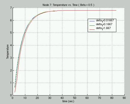
Figure 2: 1D Transient Temperature vs Time for Node 7 with b=0.5

Similar results were obtained for the 3rd node of the ten element (11 node) problem.

To further analyze the thermal solution, the same ten element structure was run with a b=0.25, which is no longer unconditionally stable. The result obtained for node 7 of the structure is:

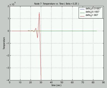
Figure 3: 1D Transient Temperature vs. Time for Node 7 with b=0.25

The figure above shows that the result becomes highly unstable for a larger Dt (1.667). Figure 4 shows only the smaller two Dt which appear to generate the same result

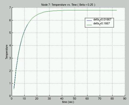
Figure 4: 1D Transient Temperature vs. Time for Node 7 with b=0.25

( only the smaller two Dt are plotted )

From the results of the runs, one can conclude that the code appears to be working correctly and that the affect of b is important for the stability of the problem.

3.0 1D Transient Structural Problem

3.1 Theory

The transient structural problem was also implemented using a direct integration method known as the Newmark Method. The method is based on the following equations for the displacement and velocity of an element:

(4)

(5)

substituting the above equations into the second order direct integration equation #1 at time (n+1)*Dt yields:

(6)

which is implicit if b is not equal to zero. Stability is determined by the selection of g and b as seen in the table below:

Table 2. Beta & Gamma Schemes

g < 1/2	unstable
2b >= g >= 1/2	unconditionally stable
g >= 1/2 & b < 1/2	conditionally stable

The time step can be calculated using the equation (7) below:

where (7) & (8)

3.2 Code Implementation

As in the transient thermal problem, the transient structural problem is implemented in one-dimension. The user selects a beam structure composed of several elements. The elements are defined by their density, length, cross-sectional area, young's modulus and imposed traction on its surface. In addition fixed displacement and constant applied force boundary condition can be assigned to the corresponding nodes of the structure. In the input file a boundary condition of type 0 refers to an imposed displacement that is specified in the input file. If the boundary condition is of type 1 then an imposed force is applied to the specified node. As before, the number of time steps determines for how long the calculations will be performed. The time step used is given by equation (7), while the constants g and b are based on the type of scheme the user selects.

A copy of the actual code is attached to the back of this paper.

3.3 Graphical User Interface

The structural program also has a separate graphical user interface in which the user can specify the 1D field and any boundary condition.

Figure 5: Graphical User Interface for 1D Transient Structural Code

The interface is called display_struct.tcl and can either be started with the command: wish display_struct.tcl or if the file is “executable” then simply typing display_struct.tcl will bring up the program. This interface is similar to the thermal problem interface. Run parameters including the number of time steps, the time step increment, Dt, b and g are selected first. Next the elements are defined and finally the boundary conditions are imposed. The user can impose one of two boundary conditions: either a fixed displacement or a fixed force. If the user selects a fixed displacement then the “BC type #” should be set to 0, otherwise if the user selects a fixed force then this value should be set to 1.

The code is run by pressing the “Run” button which will also generate a corresponding input file in the text box on the right side of the interface. Also, as with the thermal interface, the user can view an animation of the displacements over time. Once the code has finished it’s calculations the user simply presses the “Animate” button which will show the nodes moving accordingly to the result for the specified inputs.

A copy of the actual code is attached to the back of this paper.

3.4 Results of Test Cases

The 1D transient structural code was also tested for a beam of ten 1.0m long elements. The left side of the beam was fixed while the right side had an imposed force. The first test case involved and unconditionally stable method with g=0.6 and b=0.6. Figure 6 shows the result of the analysis on node 3 of the structure. The displacements are identical of the varying Dt values.

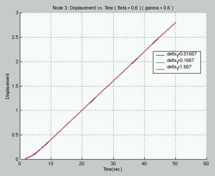
Figure 6: 1D Transient Displacement vs. Time for Node 3 with g=0.6 and b=0.6

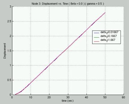
Figure 7: 1D Transient Displacement vs. Time for Node 3 with g=0.5 and b=0.0

For the second case the method selected corresponds to the central difference method with g=0.5 and b=0.0. The results (see figure 7) are identical for the varying Dt values.

The final test case was for an unstable method with g=0.52 and b=0.5. The results were as expected. The largest Dt of 1.667 sec had a very oscillatory solution that appeared to diverge with time. The results are clearly seen in figure 8.

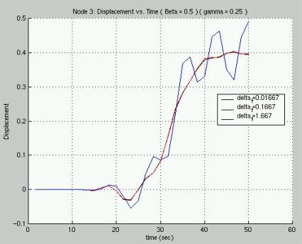
Figure 8: 1D Transient Displacement vs. Time for Node 3 with g=0.25 and b=0.5